Dealing with avoided-crossings
In general, the approach of eigenspace dynamics is severely hindered by failure in numerically obtaining reliable K matrices around avoided-crossings.In order to get the electronic dynamics right, K+- has to be correctly calculated. This turns out to be very difficult for an N X N system when the electronic dimension N is large (>200).
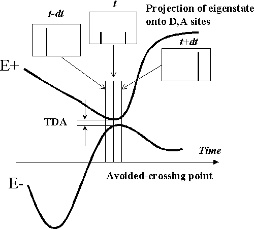
Why is it so difficult to get correct K+-? Because in proximity to an avoided-crossing point, the eigenstates |-> and |+> changes dramatically. Before avoided-crossing, they may be composed of only D/A character, exactly at avoided-crossing, they consist of equal amounts of D and A characters, and after avoided-crossing, they are composed of only the other D/A character. (see the picture below.) The time for such a change is determined by the magnitude of the energy splitting at the avoided-crossing point, namely, the non-perturbative superexchange coupling. If the coupling is very weak, the crossover time will be very short, because only a tiny amount of dynamical fluctuation of the protein is enough to push the system off resonance. In a real MD simulation, the crossover time is normally of the magnitude of less than 10-6 femtosecond. As a result, if we use a steplength of about 10-1~-3 femtosecond when computing the K+- for a weakly coupled system, most likely we would miss the crossover region, and get a false K+-(tAC) (which is usually much greater than it should be---K+-(t) thus calculated looks like a delta function with the peak at tAC but in reality K+-(t) should NOT have any peak if we zoom in to the appropriate level of time steplength).
A worse thing is that even in an adequately strong coupling case,
the non-perturbative superexchange coupling can at some points be very
small (though its statistical average value is not small), thus the
problem may happen in whichever coupling case. The worst thing might
be that it could be extremely hard to know where the AC point is exactly
at if the coupling is extremely small, if there is no other way of
getting it than zooming in and searching along the MD trajectories of
|+> and |-> inch by inch (this job is much more computationally expensive
than finding the AC point by tuning the D, A energies for a static system,
and it has to rely on the cubic spline functions).

The origin of the avoided-crossing problem: Numerical calculation often gets wrong K+-(tAC) when the crossover time dt is far smaller than the K-slice timelength.
The consequence of miscalculating K+-(t) is
that the propogation will no doubt be wrong at the crossovers (which
happens to be the most important moments for electron transfer),
and because the propogation at longer time is a cumulative function
dependent on its history, once it goes wrong at a crossover, it
will keep the mistake for the remaining time of simulation.
A postscript file about the relationship
of the accuracy of the propogation dynamics with the K matrix steplength
(what I call slice length) well explains this. There are at least two
avoided-crossing events in the case of this picture. Both resulted in
a sudden rising of PDA(t) because of overestimating
K+-(tAC) (which might mean the increment we
have chosen in the calculations is greater than the crossover time).
Unfolding dynamics from eigen space to local space
For strongly coupled systems, the eigen dynamics approach has proven
successful in reproducing the exact dynamics and elucidating the
effectiveness of the two-state approximation. Here is a
postscript plot
about the success.
Code: dyneigen.f
© 2000, Qian Xie